
Your cart is currently empty!
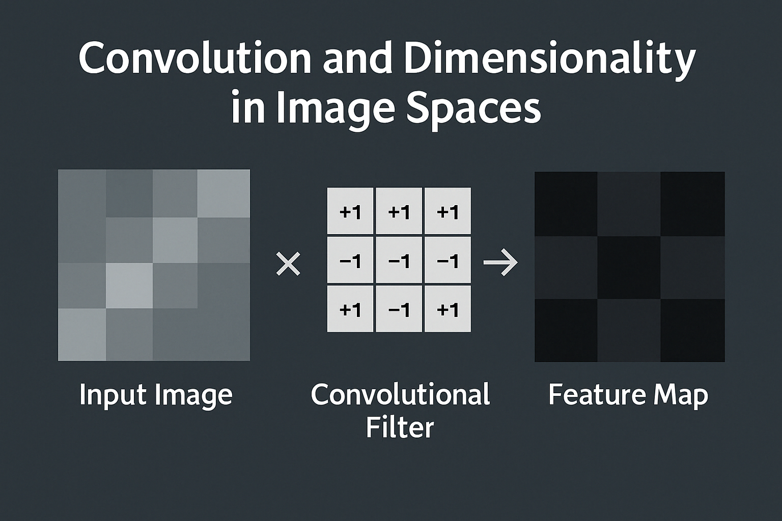
Image as a High-Dimensional Space
For a \(224 \times 224\) grayscale image:
- It resides in a 50176-dimensional space (flattened array of pixel intensities).
- Each pixel represents one dimension, so the space is vast and sparse, with most random points in this space being unstructured noise, not realistic images.
If the image is RGB \(224 \times 224 \times 3\):
- The space has 150,528 dimensions, further increasing its complexity.
What Convolution Does
Convolution applies a filter kernel (e.g., \(3 \times 3\), \(5 \times 5\)) over the image to extract local patterns such as edges, textures, and shapes. This operation reduces redundancy in the data, focusing on meaningful features.
Key Properties of Convolution
- Spatial Extent Reduction: The size of the output feature map depends on the kernel size, stride, and padding:
\( \text{Output size} = \frac{\text{Input size} – \text{Kernel size} + 2 \times \text{Padding}}{\text{Stride}} + 1\)
Convolutions often reduce spatial dimensions, especially when stride > 1 or padding is not used. - Channel Expansion: Convolution can increase the number of feature maps (channels), depending on the number of filters used.
- Dimensionality Transformation: While convolutions do not inherently „flatten“ the data, they transform the input into a new representation by aggregating local regions into lower-dimensional structures.
Does Convolution Reduce Dimensionality?
- Yes, Spatial Dimensionality:
- Each convolutional layer reduces the spatial extent of the input (height × width) if no padding or strides > 1 are applied.
- Example:
- Input: \(224 \times 224\)
- Convolution: \(3 \times 3\) filter, stride 1, no padding → Output: \(222 \times 222\)
- Stride 2 would halve the dimensions, \(112 \times 112\).
- No, Overall Dimensionality May Increase:
- Convolutions often expand the depth (number of channels) by applying multiple filters, transforming the input from a single-channel image (or 3-channel RGB image) into multi-channel feature maps.
- Example:
- Input: \(224 \times 224 \times 3\) (RGB image = 150,528 dimensions).
- After convolution: \(112 \times 112 \times 64\) (with 64 filters, ~802,816 dimensions).
Why Dimensionality is „Reduced“ Conceptually
Even if the raw dimensionality (total number of elements) increases, the convolution operation reduces the effective dimensionality:
- It enforces locality, focusing on relationships between neighboring pixels rather than treating all dimensions as independent.
- It reduces redundancy by extracting structured features (edges, corners, textures) and discarding irrelevant noise.
- Higher layers of the network aggregate local features into global ones, collapsing the data into progressively lower-dimensional feature spaces (e.g., via global average pooling or fully connected layers).
Striking the Balance
- Early layers in a CNN might increase the raw dimensionality due to channel expansion, but the feature representations become increasingly compressed as layers go deeper.
- Pooling operations (e.g., max-pooling, average-pooling) explicitly reduce spatial dimensionality, complementing the convolutions.
Final Dimensionality
At the end of a CNN:
- The data is often reduced to a compact vector in a much lower-dimensional space. For example:
- Input: \(224 \times 224 \times 3\) (150,528 dimensions).
- Final feature vector: \(1 \times 1 \times 512\) (512 dimensions).
Conclusion
Convolution reduces the effective dimensionality of the image space by compressing and summarizing local patterns into structured feature representations. The raw number of dimensions may increase in early layers due to added channels, but the spatial and informational complexity of the data is greatly reduced, especially in deeper layers of a CNN.